Find records in multiple sheets

This lesson will explain to you how to use query function to search specific record from multiple sheets.

According to our example we have three sheets.These sheets have been named as Main,Sales and Purchase.We have Included search box in "Main" sheet.Please see the following screen shot.

image 01

We have to write query function in cell G5.Once invoice number is entered to F5 cell then query will search matching  invoice number  from Sales sheet as well as Purchase sheet.This query function can be used to search more than two sheets.

I used following query function to search records in a multiple sheets

=QUERY({Sales!$A$3:D;Purchase!A3:D}, "Select Col4 Where Col1 contains '"&F5&"'",0)

Here

• Sales!$A$3:D means the Sales sheet
• Purchase!A3:D means the Purchase sheet
• Col4 means the "Invoice Amount" column
• Col1 means the "Invoice Number" column
• '"&F5&"'" means the cell number of search text box reference in main sheet

                                                                                           image 02

You can search any records from multiple records by following this method.

Source
Link to sample sheet
 https://docs.google.com/spreadsheets/d/1ttQL5ioAhGSHckyTGB7dlhDzxTVj0I5njgOlA76F8vU/edit?usp=sharing

VLOOKUP in google sheets

Google Sheets VLOOKUP - syntax and usage.

 The VLOOKUP function in Google Sheets is designed to perform a vertical lookup - search for a key value (unique identifier) down the first column in a specified range and return a value in the same row from another column.

Function Syntax

=VLOOKUP(lookup value, table range, column number, [true/false])

• Lookup value. The cell that has the unique identifier.
• Table range. The range of cells that has the identifier in the first column, followed by the rest of the data in the other columns.
• Column number. The number of the column that has the data you’re looking for. Don’t get that confused with the column’s letter. In the above illustration, the states are in column 4.
• True/False. This argument is optional. True means that an approximate match is acceptable, and False means that only an exact match is acceptable.

Please see following example to understand the application of vlookup function.
Example # 01

Explanation
The function we have used in the above screen shot is as follows;

=VLOOKUP(A3,$H$3:$I$13,2,false)

In this example A3 means lookup value cell.$H$3:$I$13 range is the table range.Numbr 2 means column number.According to the range table it is second column,if not i column according to our example.
Please carefully study above image.There we have two tables.One is called Main table and the other one is called lookup table.Then what we need to do here is to math ID column with the lookup table.In that way we can combine tables and extract details from one anther.

Example # 02

For this vlookup example we can give a named range,it makes easy our task when it comes to a large database.

To give a named range please follow this path:

• Go to Data tab and click on it.
• From the drop down list select Named ranges

Then you can see a form as shown in the below image and give a suitable name for your Named range.After that give the table range then click on the ok button.According to our example Data range is as follows;

A2:F13 

In this example we expects to get student names for student IDs.There we have entered student ID numbers to A16 column and we want to get the student names to B16 column.once you entered the vlookup function to A16 column and drag it down until the A26 column to get details for other rows too.

Limitations or vlookup function

1. Google Sheets VLOOKUP cannot look at its left, it always searches in the first (leftmost) column of the range. To do a left Vlookup, use Google Sheets Index Match formula.
2. Vlookup in Google Sheets is case-insensitive, meaning it does not distinguish lowercase and uppercase characters. For case-sensitive lookup, use this formula.
3. If VLOOKUP returns incorrect results, set the is_sorted argument to FALSE to return exact matches.
4. When is_sorted set to TRUE or omitted (Vlookup with the closest match), remember to sort the first column of range in ascending order.
5. Google Sheets VLOOKUP can search with partial match based on the wildcard characters: the question mark (?) and asterisk (*). Please see this Vlookup formula example for more details.

Creating reports based on the date ranges

It is time to learn how to create a report based on the custom date range with the help of  query function in google sheets.This will be a very helpful lessons for every one who loves to work with google sheets.

image 01

Assume that we have a large data table as shown as above image 01.So if we are able to select the data according to a given date range then it will be very useful in our day today activities.To do this we have to design a report template as shown in the below table(image02).

image 02

Query is entered to the A5 cell and we use C3,D3 cells to input dates.For date cells we can use date picker to select dates easily.

For A5 cell we enter following formula.

=iferror(query(Data!A2:F,"where A >= date'" & text(C3,"yyyy-mm-dd") & "' and A <= date'" & text(D3,"yyyy-mm-dd") & "' "))

image03

Once we entered the query to A5 cell,it is time to give desired date range to C3 & D3 cells.Then query extract details from "Data" sheet according to the given date range.

Google Sheet reports using query function

Query function in Google Sheet

This blog post explains to you, how to deal with the quarry function in google sheet.Actually quarries play important role in a every database.So when it becomes to google sheet also same.Lets start our work.

image 01

Basically,we use above data table to learn google query function

We need to assign a name for our data table under name range,before doing this we have to highlight whole table first.

                                                                                                 image 02

Then you have to assign name for your data table under the Named  ranges.So this makes our work easy.To do this you have to click on the data then select Named ranges from the drop down menu.

image 03

image 04

According to this we have Named our data table as  "INVOICE" .For Named ranges you have to give this name.

In Google sheets we use the Google Sheets QUERY function and write our SQL code inside this function.So,we'll enter all of our SQL code inside a QUERY function.

Select all data using SQL query function

image 05

By using following query we can select all data from the source table.

=QUERY(INVOICE,"SELECT *",1)

We used above query to generate new data table.According to this query it selects all the details from our original table.when it comes to normal SQL there is a difference.

Under the general SQL function we use "From INVOICES".Therefor the difference you should notice is we do not use FROM clause with the Google Sheets query function.

From above we learned how to get all table details at once. Now it is time to learn the way of selecting specific column tables.

Selecting specific columns using query function.

If we want to select specific details from the example data table above formula can be used.Assume you need to take Invoice number and the Invoice amount from the above table you just needs type following query function to get this;

image 6

=QUERY(INVOICE,"SELECT B, D",1)

To select Invoice date,Invoice amount columns we used above query. 

if we explain above query further "INVOICE" is the name given to the main table.It means we have already given this name to Named ranges.Then "B" and "D" are the columns from main table. 

Next,try to select Invoice No and Invoice Amount from the main table.To do this query should be designed as follows;

=QUERY(INVOICE,"SELECT A, D",1)

image 07

Look at the image 07,it shows the result of the query that we have designed recently.

How to authorize google script?

You have to pass following steps to authorize google script.

Step 01

click on the Review Permissions button from this menu.

Step 02

choose your account from this window

Step 03

Click on the "Advanced" link 

Step 04

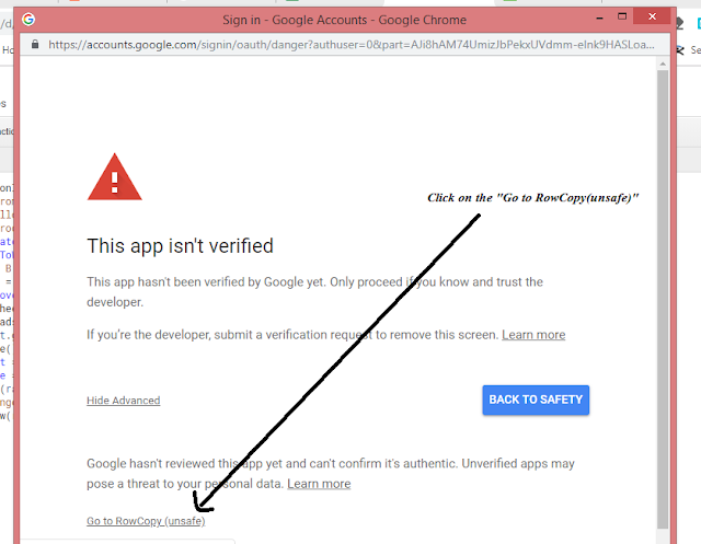
Next click on the shown link from this  arrow head.

Step 05 (Final Step)

Click on the "Allow" button to finish the process.

IMPORTXML function to get images from websites

Image extraction using IMPORTXML formula

In this article we’ll work through a similar scenario and explain how to use the IMPORTXML  function of Google Sheets to import how many likes our Facebook page has and how many followers our Twitter page has. This function doesn't update on its own by default so we've written a script that we'll explain how to adapt to ensure your data is kept up to date. 

The syntax of the ImportXML function is:

=IMPORTXML(URL, query)

URL

The URL of the page to examine, including protocol (e.g. http://). The value for URL must either be enclosed in quotation marks or be a reference to a cell containing the appropriate text.

query

The XPath query to run on the data given at the URL. Each result from the XPath query is placed in its own row of the spreadsheet.

In this blog post it is expected to explain how to import images from websites.

To take images from webites you have to use IMPORTXML function as follows in google sheet.

=IMPORTXML(A2,"//img[@class='dynamic-image']/@src")

Above function the word "dynamic-image" has used to extract images from websites.This is vary when it comes to different sites.

We use following URL to grab images from web site.

https://www.banggood.com/Soloop-328pcs-21-Polyolefin-Halogen-Free-Heat-Shrink-Tube-Sleeving-5-Color-8-Size-p-969574.html?rmmds=flashdeals&cur_warehouse=CN

image 01

This is the web site we use to extract the images to google sheet;

https://www.banggood.com/Soloop-328pcs-21-Polyolefin-Halogen-Free-Heat-Shrink-Tube-Sleeving-5-Color-8-Size-p-969574.html?rmmds=flashdeals&cur_warehouse=CN

To extract the image from the above website we used following google sheet function;

=IMPORTXML(A2,"//img[@class='dynamic-image']/@src")

according to the above function word 'dynamic-image' has been used as a key word to extract image.This can be extracted from the page source.To get the page source right click on the website and then select the view source from the menu.Then you can select desired word easily.Please see below image,it will show you how we select word 'dynamic-image' for our image extraction formula.

image 02

Summery
Following formulas had been used to fill shown table in image 01.

Link to deal -

https://www.banggood.com/Soloop-328pcs-21-Polyolefin-Halogen-Free-Heat-Shrink-Tube-Sleeving-5-Color-8-Size-p-969574.html?rmmds=flashdeals&cur_warehouse=CN

Website Name -

=REGEXEXTRACT(A2,"\.(.*?)\.")

Item title -

=IMPORTXML(A2,"//strong[@class='title_strong']")

Item Price -

=IMPORTXML(A2,"//div[@class='item_now_price']")

Image URL extraction formula -

=IMPORTXML(A2,"//img[@class='dynamic-image']/@src")

Image -

=image(E2)

Please click this link to go to sample spread sheet.